The Foundation of Distribution Efficiency: Analysed your Order Profiles Lately?
Several recent trends – like smaller, more frequent orders, faster delivery windows and value added services – can wreak havoc on distribution operations. If you haven’t taken a step back to analyse the impact of these changes, your well-oiled distribution machine may now be a rusty clunker. And with distribution playing an ever more important role in influencing customer satisfaction, it may be time to take another look at where you can improve. The place to start is with your order profiles.
Death by 1,000 cuts
Order profiling is often done as part of the DC design process. Companies then operate under those profiles for years while their business and customer requirements change. It’s a death by 1,000 cuts. No single blow is fatal. But in the end the operations are inefficient, costly and not delivering the service level your customers expect.
If that’s the situation you’re in, the first step is to assess where you stand relative to your performance metrics. Questions that arise when reviewing your performance may include:
· Are orders shipping on time? What level of service is required?
· How long does it take to process orders (from inventory allocation to shipping)?
· What is the true cost of fulfilling orders using the current processes?
· Where are my bottlenecks? Do the operational processes and capacities match the order profiles?
· If I were to fulfill orders according to my customers’ expectations what would I have to change?
· What capacity changes are required to successfully fulfill current order profile requirements?
· What do my business partners require of my distribution center?
When you know the answers to these performance questions you can then focus on the impact of analyzing your order profiles. That will help you answer questions like:
· What percentage of my orders are similar?
· What items are most often ordered together?
· When are my peaks and valleys?
· What is the effect of seasonal highs and lows?
· What is the effect of promotional campaigns?
· Is my inventory positioned correctly?
· Where are the constraints in the supply chain, and how can we remove them?
· Armed with that knowledge, you can start to make decisions about the changes in processes, capacity, throughput and inventory that will yield greater efficiency and the flexibility to adapt to both your internal customers’ (merchandising, store operations, etc.) and external customers’ needs. But where do you begin to understand your order profiles?
10 Steps to Understanding Order Profiles
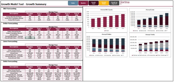
1. Profiling starts with collecting historical data, assessing current performance and understanding business partner requirements, as well as projections and growth assumptions. Analysis of historical profiles helps you understand what actually happened. But historical information can be and often is artificially constrained, meaning that it doesn’t indicate what needed to happen to deliver on time with the right product. If your past performance is less than desired, it’s also important to understand what should have transpired over the same historical timeline. You must compare should have shipped dates with actual shipped dates to understand what capacities were needed to be successful. And projected future order profiles are needed to create throughput requirements for each operational area. Growth projections and requirements should come from the business leaders including merchants, buyers and planners in your organization to help you understand where the business is trending, company goals, revenue targets, inventory plans, etc. Be sure to identify a specific time horizon associated with these forward-looking perspectives. Having seasonal, promotional, near- and long-term perspectives provides better insight about the impact to your operations and the degree of change caused by the future profiles discussed. A typical growth model might show sales, unit and SKU growth by year, by channel, by product type, class or sub-class (as detailed as can be provided by the business). Look at sourcing and demand growth patterns to determine which SKUs, categories or sub-classes might be good candidates for vendor direct shipments, thus bypassing your DCs, creating efficiencies, service improvements, customer satisfaction and lowering costs.
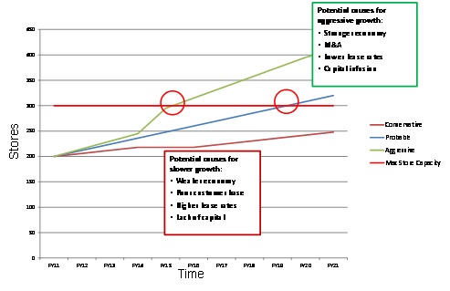
Assumptions about growth are highly subject to change, so we suggest that you both confirm your assumptions with key stakeholders and consider doing a tipping point analysis as you move forward. Generally speaking, the longer the time horizon, the higher the variability will be in your projections. Identifying sensitivities and their around projections will help you to understand how your profiles might change, impacting your supply chain in an uncertain future.
An example of tipping point analysis assumptions around base growth projects is illustrated below:
Adjusted historical data should include detailed receipt transactions, inventory on-hand data (month-end snapshots), shipment transactions and order history data. As you are studying what, in most cases, can be large data sets you want to look at the data characteristics. By looking at single line orders and profile characteristics of certain product families you start to see how changes in where and how these items are stored and picked can have impact.
To handle this large transactional data set look for a tool that provides flexibility and speed to turn analysis quickly, providing shorter time to insight. The results are a more complete analysis that can be produced consistently over time to keep pace with changes to the business.
With your adjusted baseline data, performance metrics, growth projections in hand, you can then begin to understand your company’s order profiles which drives new capacity and throughput requirements. Armed with this analysis, conclusions can be drawn about how and where to make the necessary changes in your distribution operation. The goal is to drive the process from the customer perspective (metrics) backward to establish how the historical customer needs should have been met using the new capacity and throughput requirements.
2. Identify receipt characteristics. Review the data collected by graphing a trend line, noting total units, lines, SKUs and inbound orders. Begin your analysis by understanding the mean (average) and standard deviations (+1, +2, +3 above the mean) for units, lines, orders and trailers. Standard deviations help you evaluate design requirements. Designing to peak may be too much and designing to the average is almost never adequate. Step back and ask some questions:
· Do you see expected seasonality trends? How often are you receiving seasonal SKUs, is it all at once or a continuous flow over the course of the season?
· Do you see expected peaks and valleys, or were there abnormal events during your baseline period?
· What about your supplier base or buyer behaviour is driving this profile? Is it something recurring that you can plan for?
· Is there an opportunity to use this data to educate the organization and potentially adjust a requirement? Should you segment the peak seasons?
· Are the spikes long or frequent enough that they should be your design threshold?
· By sharing this information with the rest of your organization, is there an opportunity to engage in collaborative planning across sales and procurement?
3. Identify shipment characteristics. Outbound shipment characteristics tell us more about customer demand patterns. Again, if you are operating in a constrained environment the historical data should be based on scheduled ship dates to understand the true demand and capacity requirements. So create a graph like the one below and notice how many times you exceed your design standard. In both receipt and shipment analysis, be sure to track dates so as to identify the number of occurrences by date and double check to make sure there are no other anomalies in the data, such as a one-time promotion. Pause to review, asking similar questions as in the receipt profile analysis.
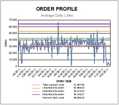
Outbound Lines Order Profile
In this example of an outbound order lines profile, there was an average of 31 million orders per day with a maximum of 66 million. The largest spike exceeds 3 standard deviations and there are several drops in line volumes. Along with this high variability, there are service requirements that must be addressed. As the saying goes, “you don’t build the church for Easter Sunday,” balancing between service requirements and variability in this example you would likely want a design based on +1.5 standard deviations.
4. Identify inventory characteristics. Depending on your company’s business rules, this data may not be available in as much detail. However, for financial purposes, inventory data is typically available as a month-end snapshot of inventory-on-hand. Capture this data for 12 months in as much detail as is available. Determine your days on hand values and average inventory turns. Review inventory profiles by product groupings such as by category or other grouping where inventory characteristics are similar and perform a comparison to your SKU velocity profiles. Inventories may move differently throughout the year depending upon what they are. For example, snow tires may sit in inventory through the summer but have several turns within 2-4 months of the year during winter. Consider a few questions in this analysis such as:
· Do the velocities of some product groupings suggest large or small storage media positions?
· Do the cubic velocities of some product groupings suggest higher productivity pick media?
· Should the seasonality drive larger pick locations for 2-4 months of the year? (snow tires)
· How do these findings compare to your operations today?
· As you’re going through all of these profiles and your company operates in a multi-channel environment, separate data by channel (i.e., retail vs. wholesale vs. eCommerce). Even if working within a multi-channel DC, ask yourself whether the profiles behave similarly at the same time periods.
· If so, does this amplify your spikes and valleys? If not, do the complimentary profiles create an opportunity to converge channels into a multi-channel operation?
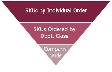
5. Analyse current SKUs and SKU velocities. Break your SKUs into deciles or ten percent increments, in descending order based on number of units sold. A slightly modified version of the Pareto’s principle still applies wherein 20-30 percent of your items generate 70-80 percent of your volumes. It’s also valuable to understand these decile SKU velocities by department or category.
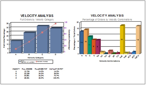
Order Completion Profile by SKU Velocity
Velocity analysis should include line activity by SKU velocity, where ‘A’ SKUs are your fast movers and ‘E’ SKUs represent zero movement for the modelling period. This tells you which SKUs are responsible for the majority of the picking activity. In this example, ‘A’ velocity SKUs are ordered by themselves 14% of the time and yet SKU velocities ‘A’ through ‘D’ are ordered together 18% of the time. This means you need to be able to get to the slower velocity SKUs to complete orders, but does not necessarily mean they need to be competing for valuable real-estate. This will impact layout and slotting efforts.
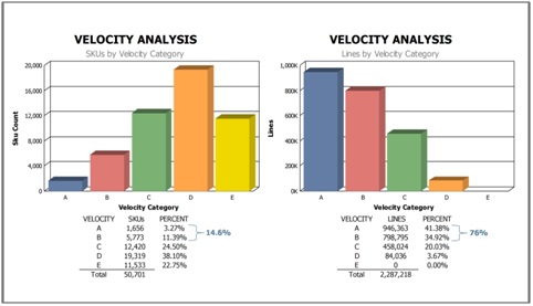
Lines, SKUs
Line activity by SKU velocity shows which SKUs are responsible for the majority of the picking activity. In the example on the left, ‘A’ and ‘B’ velocity SKUs represent almost 15% of the total SKUs and account for 76% of the line activity. It’s also important to recognize the quantity of ‘E’ SKUs and investigate whether this represents a new season’s inventory that hasn’t started moving yet or simply items that need to be removed from valuable storage space.
6. Determine product cube. Depending upon the handling type in your operation, identify each item’s case, pallet and product cube. Depending upon your processes and how products move through your operation, this may be different for receiving versus storage versus shipping. In other words, if you’re de-trashing, consolidating or repacking receipts, the cubic volume received may be different than the cubic volume stored and shipped.
7. Review operational material flows. Outline high-level material flows. Detailed SOPs are likely not necessary and too detailed for this analysis. One-line material flows are perhaps too high-level and not sufficient for meaningful discussions with your team. Following the SCOR framework made famous by the Supply Chain Council, a process flow at level 3 should be more than adequate, and you can roll it up based on your needs easily. Whether you use SCOR or an alternate process mapping method, a good rule of thumb is to document sufficient level of detail so as to facilitate discussion regarding volumes (units, lines, orders) as they flow through your operation. You’ll want to discuss how the above profiles are impacting each of your facilities at an operational process level, whether they are sufficient or need to flex differently based on changing customer expectations, etc.
8. Review productivity summaries. Review UPH, CPH, PPH or other productivity metrics you track. Break these productivities down by product category and process relating them to your operational process flows. It is important to create capacity and throughput models as a way to check productivities and understand constraints. Pause to discuss a few questions with your team:
· Which areas have lower productivities and why?
· Do these areas present capacity constraints?
· Could process or technology changes improve productivities?
9. Understand operational costs. Break down your cost statement or profit and loss (P&L) into the flows captured to show hours and volumes per process and thus calculate costs per unit throughout your operation function by function or flow by flow. Analyse for any spikes and valleys in the CPU. Consider the reasons for any spikes and what can be improved or learned to apply elsewhere with questions such as:
· Which areas have high costs?
· Is it in part due to the order profiles or perhaps product category cube?
· Are these value added processes based on customer requirements or based on a cost analysis?
10. Apply growth. Using the growth projections solicited from the business stakeholders; apply your growth appropriately to your adjusted baseline data profiles. Extrapolate forward and you should be able to begin to answer questions such as:
· Can I handle the average receipts per day, standard deviations +1, +2, +3 and peak throughout the planning time horizon?
· Can I process the average shipments per day, standard deviations +1, +2, +3 and peak through the planning time horizon?
· What is the operating plan for volume that exceeds the plan? Are there alternate flows and processes in place for handling excess volume?
· Do I have sufficient storage, or do I need to change the storage media type based on cubic velocities and days on-hand required?
· Does my cost structure remain in line with volume growth?
· Do my processes efficiently support the demand, or can I streamline?
· What are my headcount, space and equipment needs?
· Do I have sufficient capacity throughout the planning time horizon?
When is the last time you looked at your order profiles?
No one has a crystal ball to predict the future, but one thing is for certain—customer behaviour will continue to change over time. Ideally, order profiles should be reviewed annually, but companies that operate under the same profiles for years while business changes stack up against the design of the systems and facility, create inefficiencies and increase costs and bottlenecks. Understanding and monitoring order profiles regularly is key to knowing when and where to make changes to enable growth, improve efficiency and reduce costs.
Case Study: The Value of Understanding Order Profiles
One multi-channel retailer achieved 22% savings in CPU when they made the transition to fulfillment based on order profile, but they quickly discovered the value of understanding their order profiles is more than just the cost per unit (CPU) savings. It’s enabling growth and incremental revenue by better serving their customers. And it’s the flexibility to handle future growth – no matter what channel it comes through or what season it comes in.
The company was challenged as they watched their business transform from a primarily wholesale business with some retail to multi-channel with growing retail and eCommerce channels. Allocating resources and sequencing orders in a way that kept customers in all channels happy was difficult. No fulfilment engine was flexible enough to handle the different types of orders coming through a single channel. Exception handling was becoming the rule, rather than the exception.
They knew distribution held the key to improving service, reducing costs and absorbing change. And they decided they had to view the business differently if they were going to unlock that potential. The company began to look across channels at the order profiles themselves and discovered similarities around order quantity, lines, units, SKUs, product characteristics, etc. By defining orders by their profiles instead of channels or product categories, they were able to design a couple of fulfilment engines that were flexible enough to efficiently handle all of the order profiles and still allow for growth, regardless of where that growth comes from.
Bringing all the channels under one roof meant that they could take advantage of shared inventory and labour pools as well. As mentioned, CPU savings of 22% was just one benefit. The incremental revenue from improvements in customer service and flexibility to grow will yield far greater benefits for the future. However, one of the greatest benefits is the ability to leverage the peak times across channels. Some channels are busier at certain times of the year than others. Items peak in one channel at a different time than another. Having the various channels in the same building means they are able to use existing resources to ‘smooth’ those peaks across channels.
Contributed by Carey-Anne de Goede, LGA Fortna