Advanced Demand Planning
Demand Planning (DP) is the process of creating a forecast of market demand for a company’s products or services. This is crucial for most businesses as it provides visibility into the future and drives supply. Striving for the best forecast accuracy is usually the main goal of Demand Planning. The less uncertainty there is, the better the ability to make supply planning decisions. Moreover, a better forecast accuracy can be converted to higher profits.
In this article, we would like to demonstrate why companies should strive for better forecast accuracy, what the consequences of incorrect forecast are, how to alleviate possible drawbacks and also how to improve overall forecast accuracy. This look at Demand Planning underlines the importance of capturing true demand versus sales history, discusses forecast hierarchy and the optimal forecast generation level.
The optimal forecast generation level is regarded as the cornerstone of good DP design. The “best” possible forecast accuracy is required at the hierarchy level where planning (decisions) are made. It does not necessarily mean that the forecast has to be generated at that level. Aggregation, forecast generation and disaggregation, together with the right forecasting methods, could provide for the best forecast accuracy at the “decision” level.
A proper set-up of composite forecast, inclusion of non-quantitative causal factors, pre set-up analysis and post-implementation diagnostics are important DP best business practices and key factors in any successful design and the usage of Demand Planning.
Let’s examine the technical and process aspects of Demand Planning. It is vital that people with the right skill sets, knowledge and experience are acknowledged as fundamental factors for the successful design, implementation and usage of a Demand Planning solution.
Why Strive for Better Forecast Accuracy?
Companies very seldom realise to what extent demand forecast accuracy improvements contribute to the increase in Earnings Before Interest, Depreciation, Tax and Amortisation (EBIDTA).
Using Deloitte Consulting's simple EBIDTA gauge, you can estimate how a relatively small improvement in forecast accuracy may translate to a substantial EBIDTA increase (see Figure 1).
The tool incorporates the dependence of EBIDTA on service levels, forecast accuracy, lead times and replenishment periods. It conservatively assumes that changes in EBIDTA are only due to the reduction in inventory holding costs, which are estimated for an average South African company to be 35%. The holding costs include cost of money, warehousing, insurance, potential wastage and handling costs and are calculated as a percentage of the inventory value if it is kept in a warehouse for a period of one year.
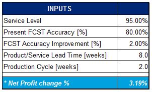
Figure 1: EBIDTA dependence on forecast accuracy improvements
Assuming a 95% service level, eight-week lead time and two-week replenishment cycle, and a 3% increase in forecast accuracy from the base of 80%, causes an EBIDTA increase of almost 5%, as illustrated.
The gauge shows the direct EBIDTA improvements based on inventory savings only. The other indirect advantages of forecast improvements address the following shortcomings of forecast error:
· Incorrect Raw Materials (RM) inventory in wrong places.
· Excessive warehouse costs.
· Inaccurate production scheduling (leading to production yield loss or increased costs).
· Incorrect Work in Progress (WIP) inventory.
· Excessive warehouse costs.
· Stock outs and late orders.
· Customer switching or increased safety stock levels.
· Inadequate (too small or too big) shipments and inter-depot shipments (excessive transport costs).
Measuring Accuracy Meaningfully
When measuring forecast accuracy it is vital to make sure that it is representative (appropriate) at all reporting levels.
Sometimes the market/product or combination of these means it makes sense to measure and report at a slightly higher level. By not aggregating a forecast correctly or by reporting on a summated total, you can easily be lulled into a false sense of security. Often forecast accuracy numbers on a very high level can achieve in excess of 95%; but is this an honest number?
Forecast error is first measured at the lowest level in the hierarchy (often an item or SKU level). Let’s quickly look at some forecast metrics:
· Percentage Error (PE): this is shown as a % and has a range of 0 to infinity.
· Mean Percentage Error (MPE): this is shown as a % between negative infinity and infinity.
· Mean Absolute Percentage Error (MAPE): this is shown as a % between 0 and infinity.
· Mean Absolute Percentage Error (MAPE*[1]): this is shown as a % between 0 and 100%.
[1] This is a normalised MAPE measure (i.e. range of values is from 0 to 1)
When aggregating the forecast errors of multiple items (or products) it important to ensure that the total number is representative of the true forecast error of the group. One may be tempted to aggregate the total sales/usage for a range of items and compare this to the total forecast. Depending on the level this should give errors between 0 and 10 % (accordingly the accuracy will be close to 100%). This may look very good on a forecast report but may hide the reality of the performance of the forecast as a whole by cancelling out the noise of over and under forecasted items. That is, if you were over by 100 items on one product and under by 100 items on another product in total you were 100% accurate – this is not representative.
In order to aggregate the forecast error of Percentage Error, MPE and MAPE you must average the errors of all the individual measures. This is a very dangerous option as high and low forecast items can cancel each other out and skew the total forecast error. This number can also be very misleading in the cases where there are forecasts errors greater than 100%, as they very quickly skew the data.
It is best to compare errors with a common range, i.e. a measure with a fixed minimum and maximum. The MAPE* error calculation is one such measure with a range from 0 to 100%. Averaging this number will give you a number that is always between 0 and 100% which gives a level of “badness” of the forecast.
To further calculate the forecast error accurately one should not simply average all the item level MAPE*’s scores. This will result in an insignificant item (e.g. a washer) being compared with a critical item (e.g. car chassis) with the same importance (or weighting). Ideally you would want to place a higher importance on the critical items and a lesser importance on the non-critical items using a weighted average. The result is a measure of “badness” of the items as a group at the level of aggregation.
In order to accurately report on the health of a forecast it is crucial that an honest metric is used to calculate the error (and hence the accuracy) so that the forecast as a total is compared.
The next chapters focus on some aspects of the demand planning process aiming at increasing forecast accuracy.
The Demand Planning Process and the Effects of Incorrect Forecast
Demand Planning is a process of creating a forecast of market demand for a company’s products or services. It is a facility with an extensive ability to analyse data and predict possible future trends and seasonality, add causal factors and mix them with a human input.
The human element is required to inform the system about promotions, events, allocations, new product launches, customer forecasts and many more. These are added to the baseline (system) forecast and reviewed by the whole sales team in order to arrive at a single forecast (during a demand consensus meeting) that the whole company operates to.
This stage of the process generates an unconstrained demand. What can the sales team sell? Only what the factory can produce! The unconstrained demand will form one of the inputs to the Sales and Operational Planning (S&OP) process where supply and demand is balanced. In the process, in the case of shortages, conscious decisions are made:
· Which customers do we disappoint?
· Will we work overtime or outsource to not disappoint any customers?
By virtue the forecast is almost always incorrect. The external reason being demand instability (see Figure 2) and the internal being sub-optimal demand planning design. The effect of incorrect forecast causes disruptions in all supply chain areas in a number of ways.
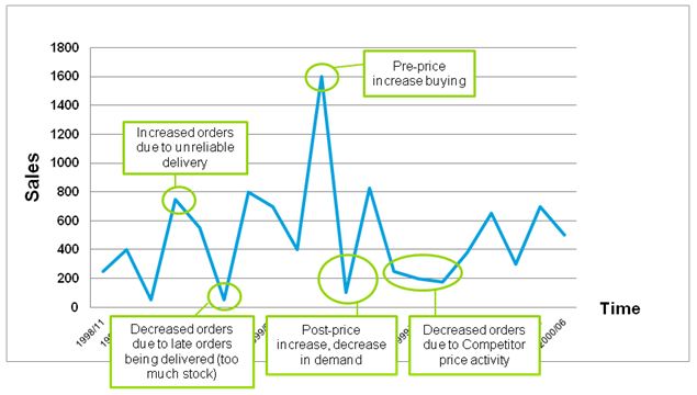
Figure 2: What contributes to demand instability?
Typically manufacturing facilities are equipped and optimised for long runs at high levels of efficiency. Significant investments are required to ensure high flexibility in supply. Manufacturing operations have to continually adapt to changes in the true demand versus what was forecasted. This approach typically results in investments in:
· Additional capacity.
· Reduction in changeover times e.g. SMED methodology.
· Additional shifts/overtime at short notice.
These changes are felt all the way through to the raw material suppliers, who also have to adapt to the ever-changing demand. They too then have to become more flexible, driving flexibility into their manufacturing and distribution processes, resulting in an increase in their costs and subsequently the raw material prices.
Regardless of their intentions, organisations never seem to have sufficient “regular” capacity to meet this ever changing demand. This is most keenly felt at the finished goods level where manufacturing capacity and distribution capacity have been locked into producing a product and shipping it to a destination that may ultimately require something else. The organisation has now been bitten twice by the same inaccuracy:
· Inventory was produced for a projected demand that never became a reality.
· Working capital is now tied up unnecessarily, on an item that may have a shelf-life or become obsolete.
Manufacturing and distribution capacity could have been better spent on producing an item that was ordered. Additional capacity (in the form of overtime and /or extra shipping) now has to be employed, in order to meet the true demand. Since the booking of this additional capacity is at late notice, it usually costs more that it did when the organisation was producing the “wrong” item. The cost is therefore typically MORE THAN twice as much as it should have been to meet the true customer demand. It will also disrupt production for pre-existing orders. The described vicious circle is also known as “bull-whip” effect.
Many organisations have opted out of this vicious cycle by choosing to buffer with additional finished goods inventory. Whilst this buffers the operations and suppliers from demand variability, it drives up finished goods inventory significantly. Higher levels of finished goods inventory exposes the organisation to increased risk of:
· High stock obsolescence.
· Shrinkage.
· Additional warehouse capacity.
With holding costs of approximately 35% of the value of inventory, it represents a significant supply chain cost component (working capital), which can be addressed starting with forecast accuracy improvements initiatives.
It is clear that there is no single comprehensive solution to all companies facing this challenge. The best approach is to determine the trade off between the increased costs of manufacturing flexibility and the increased costs associated with the holding of excess stock. The tipping point will most likely contain a combination of the two approaches. Deloitte Consulting has found that accurate business hypothesis modelling is instrumental in making this decision.
True Demand versus Sales History
Another technique used to improve forecast accuracy is to move towards forecasting based on true demand (POS data and stock-out information) versus forecasting based on sales history. This is particularly important in businesses that experience periods of peak demand and instances of stock shortages.
The following factors are prevalent in these circumstances:
· When multiple customers are calling for inventory that is out of stock; capturing of lost sales by the organisations’ order fulfilment clerks is usually very poor.
· Where alternative items are available, substitution capturing may lead to skewed demand data.
· Where there is general knowledge in the customer base that there is a short supply situation, customers tend not to call and place orders so the true demand is lost.
One method to ensure that the organisation has a better sense of true demand is by ensuring that the order-takers (be they sales reps, telesales or order fulfilment centres) implement a process for capturing back orders and lost sales orders, thereby realising the following benefits:
· Customers will continue to call during a low-stock situation as the order will be captured, thereby enhancing the organisation’s understanding of lost sales versus delayed sales.
· The organisation will get a better understanding of substitution sales versus what the customer actually wanted, and will move much closer towards capturing true demand on which to base the statistical forecast.
Forecasting at Optimal Hierarchy Level
Many organisations are obsessed with forecasting at the most detailed level possible, claiming that only at this level are they truly able to try and predict true customer demand in line with customer ordering patterns (aiming to minimise potential ‘out of stock’ situations). These are planning or ‘decision’ hierarchy levels.
To achieve this, they set up their demand forecasting applications or models to produce a statistical forecast at a SKU level right at the point of consumption. This granularity could be represented:
· By brand.
· By pack size.
· By day.
· At the end-user location.
At that granularity level the demand signal tends to be very ‘spiky’, fluctuating between periods of high demand and periods of no, or little, demand. This typically results in a highly variable forecast with low accuracy.
The other complication is that stakeholders in various business functions (marketing, sales, distribution, manufacturing, purchasing, administration, finance, etc.) plan at strategic, tactical and execution levels. They usually require forecasts at different hierarchy levels.
In all cases the planning and decisions are made based on forecasts at certain product/customer/geography/ time hierarchy levels. It is then crucial to obtain the best possible forecast accuracies at those hierarchy levels. It does not necessary mean that the forecasts need to be generated at those levels. The forecast can be generated at any level, as long as through the process of aggregation, forecast generation and dis-aggregation, the best accuracies at the planning (decision) levels are obtained. The generated forecast is a composite forecast (see Chapter 7) with judgemental inputs added at the adequate hierarchy levels (see Figure 3).
The design of the hierarchy, aggregation of historical data, reconciliation of forecasts (Figures 3 and 4), conversion between various units of measure and the identification of the optimal forecast level are vital issues to achieve the best overall forecast accuracy. The reconciled forecasts render planning (decision-making) of different stakeholders in various business functions in required timescales.
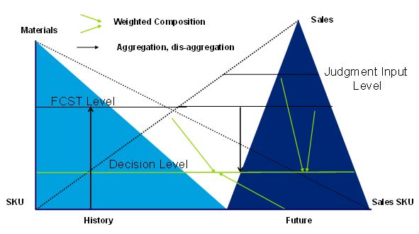
Figure 3: Input, forecast and decision hierarchy levels can be different
If any of these issues are neglected various forecasts in the company will not be accurate or compatible and will be manifested in unnecessary inefficiencies, since the demand planning creates the base for further decision making in the supply chain.
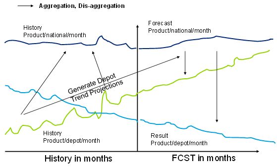
Figure 4: Aggregation, dis-aggregation concepts
The final (composite) forecast is usually a weighted combination of a univariate (time series), causal analysis (usually handled using multiple linear regression - MLR) and judgemental input.
The allocation of the weights of the components is performed based on the forecast accuracy of each component in the previous “periods”: thus the higher the forecast accuracy the bigger the weight factor. In this way the composite forecast “rewards” providers of the past top performing forecast accuracies, see Figure 5.
If the weight factors are not calculated based on “past” accuracies, then the opportunity to obtain an objective overall best forecast is limited.
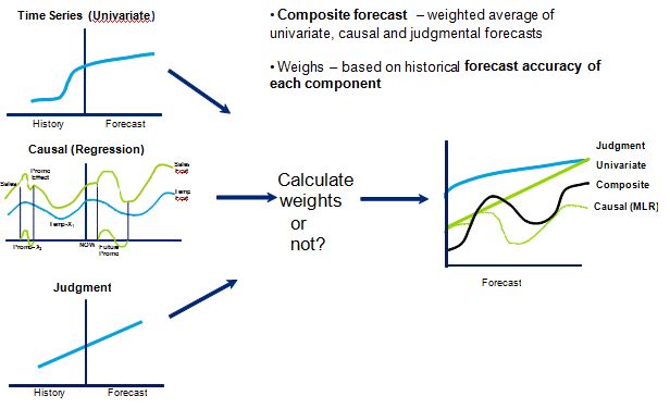
Figure 5: The composite forecast
Inclusion of Non-quantitative Events as Causal Factors
If causal analysis is one of the components of the composite forecast it normally incorporates only quantitative factors (those which can be expressed as a series of numbers, for example temperature, discount promotions, wages, etc. see Figure 6).
The technique used is based on quantifying the deviation (calculating “deviation” coefficients) of the “sales” in the past caused by a factor and assuming that the factor would have a similar impact in the future. In order to estimate the forecast the calculated coefficients are used to extrapolate the impact of the factors.
These factors include, for example, temperature, income, promotional discounts, Easter, fishing quotas, impacts of legislation and special announcements. It is often impossible to include qualitative factors, such as holidays, sport events and non-value-adding promotions since it is challenging to find their numeric representation. These factors can have a substantial influence on sales patterns and are usually planned in advance or known (promotions, events, and holidays) and therefore it would be beneficial to include them in the causal analysis.
We use a propriety method of generating dummy variables out of these non-quantitative factors, which proved to be very successful in causal analyses forecast accuracy improvements.
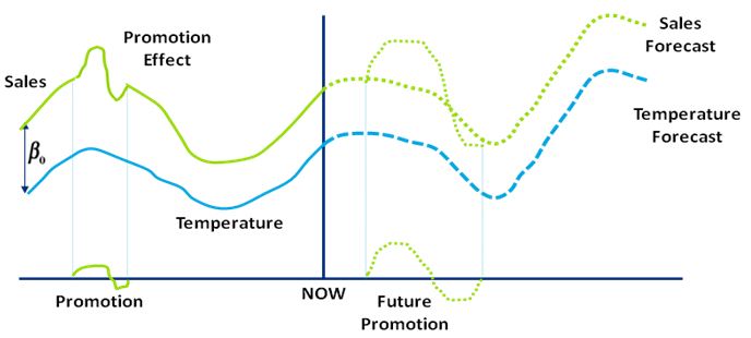
Figure 6: Temperature (quantitative) and promotion (qualitative) influence on sales
Pre-setup Analysis and Post-implementation Diagnostic
In many businesses the crucial part of Demand Planning is a statistical forecast and its accuracy, with judgemental input being on the other side of the spectrum. Generally the forecast is based on historical sales data, which is usually captured and maintained in a hierarchy structure pertaining to product; geography, key clients and time.
Therefore, the main principle of the pre-set-up analysis is to differentiate the forecast generation level and sales (or usage) data capturing level. The main reason for this is that data at those levels are usually sporadic, intermittent or exhibit “noise”. Forecasts generated at those levels do not necessarily provide the best accuracy. For these reasons, generally it is not advisable to design a Demand Planning solution based on generating forecasts at the “data capturing” levels (refer to Chapter 5).
The main principle of the sound design of a forecasting solution is based on forecast generation at the appropriate levels. Using adequate methods which, after disaggregation, provide the best accuracy of information at the hierarchy level where planning is performed (the decision level).
The proper “DP design” is crucial to attain the best accuracies. The principles of the “good” design can also be used as benchmarks for post-implementation forecast diagnostics.
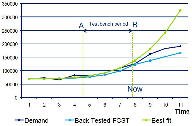
Figure 7: Back testing (ex-post forecast) concept
The pivotal aspect of our forecast diagnostic approach is the data analysis required in order to determine:
· Optimal forecasting hierarchy input (judgemental) and generation level.
· Best forecasting methods – with reference to the three possible input areas: univariate, causal and judgemental input.
· Significant causal factors and their projections into the future.
· Best methods of disaggregation, e.g. based on proportional factors, forecasts generated at lower hierarchy levels or other factors.
Whenever possible, the main criterion for selecting the best method/technique is based on back testing (ex-post forecast), Figure 7, rather than fitting the curve to historical sales (best-fit or interpolation). In many cases using the best fit provides for dismal forecast accuracy because of exponential effect of most recent history.
Many businesses believe that it should be possible to significantly improve forecast accuracy but find it very difficult to do it in practise. The Deloitte Consulting team has designed many Demand Planning solutions. The team has also assisted clients who have existing Demand Planning systems to significantly improve their forecast accuracy. The areas of improvement include processes, new approaches, fine-tuning methods and enabling advanced functionality such as causal analysis. The fine-tuning of Demand Planning is the key to realising several related benefits, such as: a well-managed supply chain, reliable client service and significant cost reduction.
Demand Planning Best Business Practices
In our experience, companies that perform Demand Planning efficiently and effectively, and therefore prosper, have many attributes in common.
These companies make use of a robust forecasting and planning system which enable their Demand Planning processes. These planning solutions are customised to their specific needs; unlike an ERP system – one size does not fit all. Demand Planning usually is a part of Integrated Business Planning.
They adhere to clearly defined processes which enhance their DP capabilities. They have a clearly defined Sales and Operations Planning process where a demand consensus is reached and fed back into the DP system where stock policy is calculated.
There is a broad view of the supply chain, not only within the organisation but between customers and suppliers too. This so called CPFR (Collaborative Planning Forecasting and Replenishment) focus allows better planning by adding input from client’s forecasting system into the DP system and feeding more information to suppliers.
These companies also manage their demand by an ABC or Pareto classification. By doing this not all forecasted items need to reviewed, only the items that will significantly influence the business. During the S&OP process only the ‘star’ items (and new items) are considered and collaborated on.
Lastly companies that successfully make use of their DP system understand that no company is too complex or too simple to forecast. Understanding the demand is a vital part of managing a supply chain.
Based on the experience Deloitte Consulting has in the supply chain industry, the key success factors for effective and efficient Demand Planning design, analysis and implementation projects have been identified:
· The active involvement of the executive sponsor will drive the DP solution from the top; this ensures buy-in from the stakeholders within the organisation.
· The understanding of the impact that forecast accuracy has on the business and knowing which measures to monitor (e.g. EBITDA).
· The quality and availability of demand and other data that influence the forecast (causal factors etc.) from a well maintained source (e.g. ERP).
· The alignment of the planning department with other departments in the business who contribute to the S&OP process (sales, marketing, manufacturing etc.).
· The skill of the personnel involved in planning and the transfer of knowledge within the business.
· The amount of continuous Demand Planning training that is provided.
 Dr Tomek Jekot, Deloitte Associate
 Stephen Povey, AngloGold Ashanti
 Clinton Houston, Supply Chain Strategy, Deloitte Consulting ZA