The world of Business Analytics (BA) continues to mature as more and more companies move beyond traditional business intelligence (BI) applications. While BI remains a key ingredient in the BA mix, BI can only deliver half-baked insights without modern modeling capabilities. Extracting actionable insights from big data requires some form of data modeling; forward-thinking to put the most profitable and strategic initiatives first.
Business
analytics is divided into 3 types of analyses:
•
Data Model/Historical Analysis – In
the context of business analytics, data models are primarily used to aggregate transactional
information and use that data for various performance management, planning and
decision-making tasks. In this way, a data model serves as an accurate
calculation engine to measure “actual” performance. Data models support what
Gartner calls “descriptive and diagnostic analytics”1 – the ability to
understand what and why certain performance behaviours or incidences happened.
Most BI tools – including advanced data discovery and visualization tools reporting
engines belong in this category.
• Predictive
Analytics/Modeling
– This modeling technique helps companies predict the behaviour of unknown key variables
that have a significant impact on the business performance. This includes
things like predicting demand (volume, prices) in various forms, input prices,
currency movements and risk (via weather or other variables). Predictive models
are also used for analysing information patterns to support tactical
decision-making; however, predictive analytics do not provide the full picture
as to what will happen to performance given a set of predictions.
• Decision Support (also referred to as business or prescriptive modeling) – Decision support helps business decision-makers predict likely outcomes if a certain plan is executed (this is often supported by predictive analytics and existing information about the business). Decision support also allows business users to run “what-if” scenarios to determine what should happen given an organization’s objectives and constraints. The most advanced decision support engines include extensive analytics features, such as forward-looking profitability analyses, marginal economics/opportunity costs (we call these Opportunity Values) and automated equation management to support broader “what-if” analyses.
There are a multitude of different types of analyses in the Decision Support category. The purpose of this article is to clarify the main approaches to Decision Support, and identify their respective advantages and disadvantages.
Monte Carlo Type Simulation versus Optimization
Business
Analytics/Decision Support modeling can be defined as mathematically simplifying
complex systems, allowing users to obtain valuable insights into the nature of
their business. These models accurately represent opportunities and constraints,
and forecast the impacts of various input variables on a business. The two main
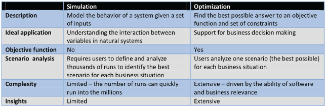
modeling approaches are Simulation and Optimization.
Simulation
provides insights based on a user-provided set of inputs. The most advanced
systems, often referred to as Monte Carlo simulations, allow users to set
parameter ranges and interval points for thousands – or even millions – of scenarios.
These systems are extremely useful in explaining various ways the natural world
works; however, simulation is not ideal for supporting business decisions.
Optimization
finds the “best possible” solution to all of the decision variables a company
identifies. This notion of “best possible” is very important: in order to reach
an optimal solution, it must be the “best” solution as determined by a given objective
(such as maximized customer satisfaction or minimized costs).
The
other half of our definition, “possible”, implies that the solution found can
actually be executed. The solution cannot violate a business constraint (constraints
could be the number of man hours available, pricing or fluctuating material
volumes).
Case in Point
To understand this better, let’s use a tangible example. Assume we are working alongside a small business that makes two candy bars: Nutcrunch and Mega-crunch. The company would like to know the most profitable product mix within constraints to raw materials and production.
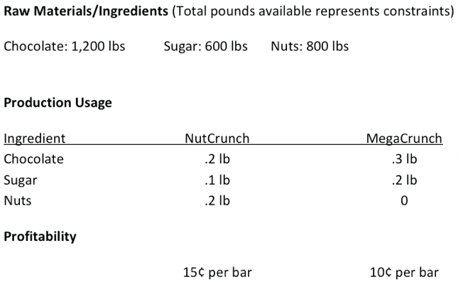
Algebraically,
this would translate into:
Profit
= .15x + .1y Chocolate = .2x + .3y
Sugar
= .1x + .2y Nuts = .2x
Where:
x = the number of Nutcrunch and y = the number of Megacrunch bars.
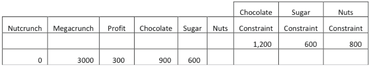
In
a Monte Carlo method simulation model, the user would enter the number of units
of Nutcrunch and of Megacrunch they wish to produce, and the model would then
report the associated profits; this is whether or not sufficient resources exist
for the desired production level.
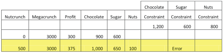
In the first simulation, the user has entered 0 units for Nutcrunch and 3000 units of Megacrunch. As illustrated, the simulation model returns a profit of $300. Additionally, both ingredients (chocolate and sugar) are below or equal to their respective constraints. In this run, the process consumes 900 pounds of chocolate; well below the 1,200 pound constraint. Similarly, sugar consumption is 600 pounds in this model, and does not exceed the sugar constraint.
Next, the user would provide new unit inputs for Nutcrunch and Megacrunch and rerun the simulation. In this run (row 2) the user inputs 500 units of Nutcrunch and 3000 units of Megacrunch. The simulation returns a profit of $375, but notice the “Error” in the Sugar Constraint column. Producing these quantities requires 650 pounds of sugar, which exceeds the 600 pound sugar constraint. Therefore, this simulation run is deemed infeasible.
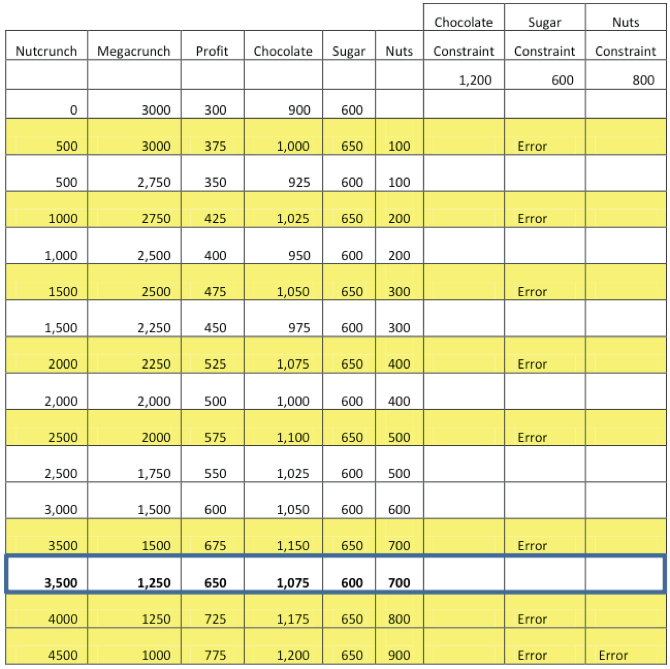
The
user continues this “trial and error” method, attempting to maximize profit while
operating within the confines of each constrained ingredient – finding their
optimal production configuration. The following table illustrates 16 total
simulations. Notice that 50% of the simulations are infeasible.
Next,
the user would review all valid outputs to determine which simulation resulted
in the most profitability. Looking at the profit column, we see that the best
production level is 3,500 Nutcrunch and 1,250 Megacrunch, which generates a
profit of 650. Using automation of parameters, ranges and relevant intervals,
this trial and error method eventually finds a solution.
A skilled user can use output from Monte Carlo simulations to determine which model delivers the greatest profit; however, simulation is not the optimal means of doing so.
In
simple problems, this approach may even come close to finding the “Best
Possible” solution, provided the user has set the right parameters. Finding the
best solution, however, is still dependent on the user’s skills and
interpretation of the results. As problem complexity increases, simulation
quickly becomes infeasible. When dealing with complex problems, a user may have
to evaluate millions of simulation runs and inputs to find the best possible
solution per scenario. For complicated problems, simulation becomes an
impractical solution in almost every case.
Optimization immediately finds the best possible solution
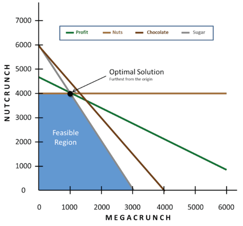
Prescriptive
modeling uses an optimization algorithm to help determine deter-mine the “Best
Possible” solution immediately. In the following graph, the optimal solution is
the unique point where the profit function intersects the feasible region of
all of the constraints, and is the furthest from the origin.
Optimization determines the optimal product mix to be 4,000 units of Nutcrunch and 1,000 units of Megacrunch. This optimizes profit at $700, nearly 8% higher than the best simulation in the previous segment.
In this situation, the user only worries about providing the minimum and maxi-mum values for the relevant constraints (e.g. raw material availability, production hours, rates and others), while the optimization finds the best possible solution.
The user only has to evaluate one run for every business scenario. As multiple business scenarios are evaluated, the user is assured they are receiving the best possible outcome in each situation. Optimization allows “apples to apples” comparisons, versus simulation in which the user might not always have the best possible answer.
The
optimization approach can calculate the Opportunity Value of relaxing
constraints, based on the slope of the lines at the intersection in relation to
the profit function. Opportunity Values represent the system-wide profit impact
an organization could see by relaxing a given constraint. Examples of this
include having more raw materials available, increasing demand or adding
resource capacity.
Monte Carlo style simulation analysis can be quite powerful, and handle an enormous amount of data; however, optimization is better suited for supporting business decision-making. Optimization quickly finds the “Best Possible” solution in a given circumstance, while also mitigating risk. Additionally, most true optimization systems can be used for simulation purposes, while simulation cannot do the same for optimization.
Contributed by: River Logic & Business Modelling
Associates (the SA channel partner for River Logic)